Data Cleaning / 2026
LyftMed Opeations Analysis I: Data Cleaning
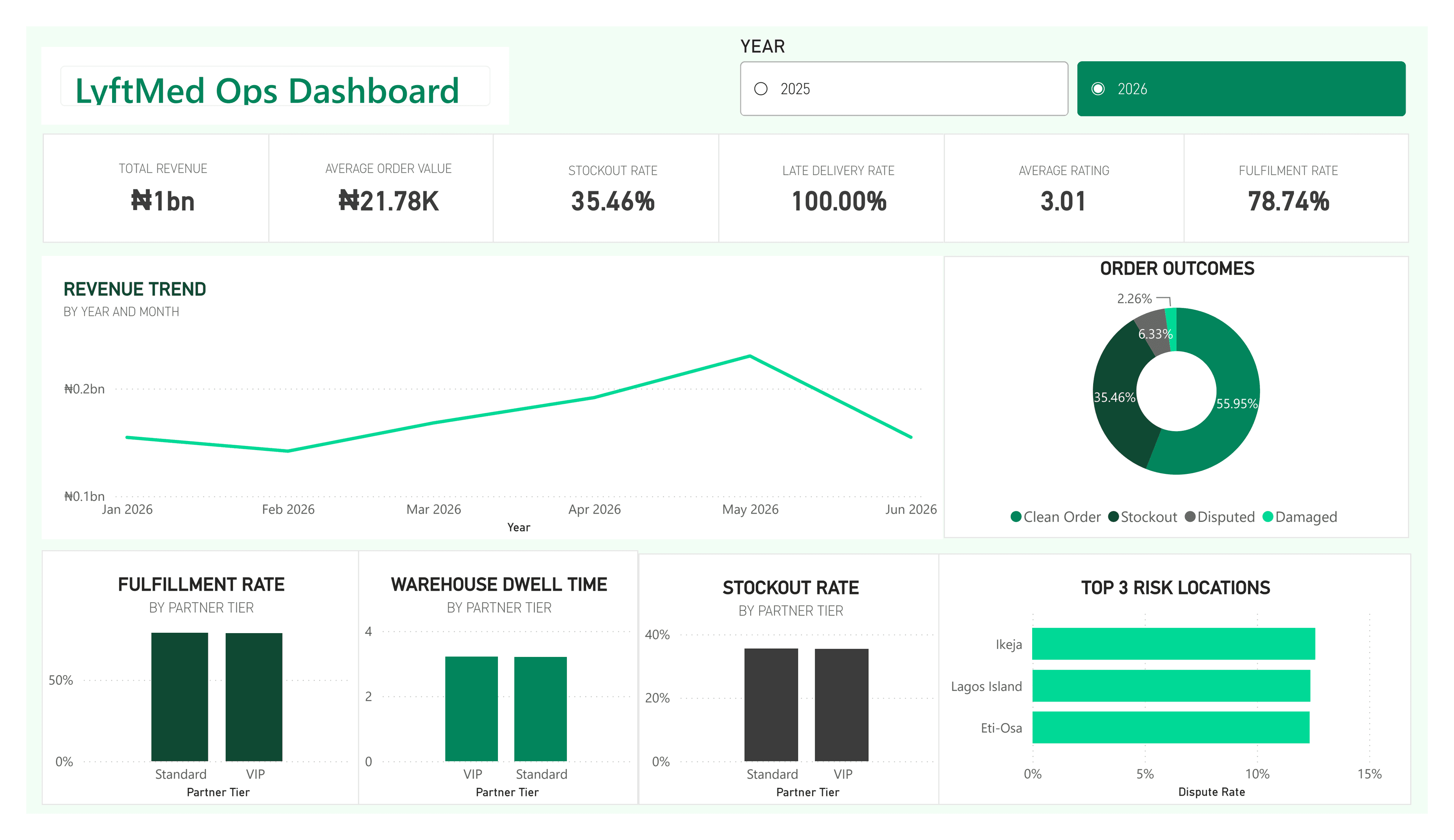
This section focuses on data cleaning, representing the first phase of a two-part project completed before the final analysis.
Background
LyftMed operates a multi-city pharmaceutical distribution and delivery network that connects customers to medicines through a network of partner pharmacies, a central warehouse fulfillment operation, and a fleet of last-mile delivery riders. Every order moves through a chain of operational stages: the customer places demand, the system checks product availability, the warehouse picks and packs the order, a rider is assigned for delivery, and the customer ultimately rates the experience.
Over the past several months, our operations and customer support teams have flagged a growing list of recurring issues. Customers are receiving incomplete orders because certain products run out of stock at the moment of picking. Deliveries are arriving late, and the delays appear to worsen during rainy periods and rush-hour traffic.
These issues are showing up in customer feedback, partner escalations, and anecdotal reports from riders and warehouse staff, but leadership does not yet have a clear, evidence-based picture of where the biggest problems actually originate. We do not currently know, with confidence, whether poor customer ratings are being driven primarily by late delivery, damaged products, stockouts, warehouse delays, or failed delivery attempts. We also cannot yet say which specific products, locations, partners, riders, or warehouse shifts are contributing the most operational and financial risk.
Business Problem
Operational issues are being felt across the business, in customer ratings, partner disputes, churn, and warehouse throughput but their root causes are not clearly isolated. Without a data-driven view, resourcing and process-fix decisions are being made on assumption rather than evidence, which risks fixing the wrong problems first.
Business Questions
Which products are frequently ordered but not fully fulfilled, and how much revenue is that costing us?
Do VIP partners genuinely receive fewer stockouts, faster warehouse handling, better fulfillment, and fewer disputes than non-VIP partners?
Is churn risk driven more by late delivery, damaged items, stockouts, or disputes?
Which LGAs generate high order volume but also high delays, disputes, damage, or stockouts?
When we run promotions, do they generate healthy incremental orders, or do they create bulk-order surges, stockouts, warehouse queues, and complaints?
Is fulfillment delay coming from warehouse capacity, worker fatigue, specific shifts, bulk orders, or stockouts?
Are late deliveries driven by specific riders, rainy season, rush hour, poor bike condition, or failed first attempts?
Methodology
Data Cleaning
1. Finding and Fixing Missing Values.
Rather than guessing where the damage was, the first script swept every relevant table (products.csv, inventorysnapshot.csv, and orderitems.csv) and flagged any row where a required column was null. This is a simple but important discipline: check every table for completeness before touching anything, so the scope of the problem is known up front. See code below:
The sweep surfaced a single root cause: one product, PRD244 (Clofazimine), was missing its category, price, tier, and coldchain classification in the master products.csv file. Because every other table (inventorysnapshot.csv, order_items.csv) pulls its category and tier labels from that same product record, the gap didn't stay contained, it propagated outward into 190 order-item rows and 1 inventory row that referenced PRD244.
Fix
Once the root cause was identified, the second script filled in the gap directly at the product level:
The same category (and tier, where relevant) label was then propagated to the matching rows in inventorysnapshot.csv and orderitems.csv, since those values are simply mirrored copies of the product master data rather than independently observed facts. Because the fix targets a known product with a known classification (confirmed via the drug name, "Clofazimine"), this is a direct correction rather than an estimate.
2. Detecting Outliers Across the Whole Dataset
The goal was to identify columns and rows with statistically implausible values, across every file, without hardcoding assumptions about what "normal" looks like for each column.
Method
The third script ran an interquartile range (IQR) check on every numeric column in every file. For each column:
Calculate Q1 (25th percentile) and Q3 (75th percentile)
Compute IQR = Q3 − Q1
Flag anything below Q1 − 1.5×IQR or above Q3 + 1.5×IQR as an outlier
This is a standard, distribution-agnostic technique that doesn't assume the data is normally distributed, and it self-calibrates to each column's own spread rather than using a fixed threshold across the board.
See script below:
Output
The result was a single consolidated report ranking every flagged column by what share of its values fell outside the fence turning an otherwise-invisible problem (buried in 11 different files) into one prioritized list. This report became the map for where deeper repair work ( like the dwell-time reconstruction below) was actually needed. See output below:
Reading through the report made it clear the flagged file/column combinations weren't all the same kind of problem.
Bucket A : extreme, but operationally plausible. These are real values a business could genuinely produce; the fence just isn't used to seeing them. An example was avgtimeperordermins with 20% outlier but on close inspection, these were possible numbers that instead may give insight to working conditions.
Rows were flagged, reviewed, and left alone they describe real operational variance, not corruption, and "cleaning" them out would have thrown away legitimate signal.
Bucket B: structurally impossible. One row on the report looked nothing like the rest: The minimum value, 3.2 hours, looks completely normal. But the 25th percentile alone already carries 74 zeroes, the median has 145, and the maximum is literal infinity. No warehouse holds a parcel for 10¹⁴⁵ hours. This isn't a heavy-tailed distribution, it's a column that broke, almost certainly from a division or overflow error somewhere upstream. With nearly 1 in 4 rows affected, this couldn't be filtered or capped the way a normal outlier could. It needed to be rebuilt from scratch, and it needed to happen immediately.
The natural way to rebuild warehousedwellhours was to compare it against each order's total elapsed time: total elapsed time = actualdeliverydatetime − order_datetime, then strip away the time spent actively processing the order, and finally the transit time, leaving dwell as whatever remained:
In theory, that's a clean subtraction. In practice, it hit two problems:
The first problem was hard to work around: transit time was never recorded at all. Nothing in the dataset captured the moment a rider actually left the warehouse. The "out for delivery" event simply wasn't a data point the warehouse system collected. So even with a good total elapsed time, there was no direct way to split it cleanly into idle dwell versus transit, since the two unknowns (dwell time and transit time) sat on one side of a single equation.
The workaround was to build a typical transit time from the data that was already known to be healthy, and use that as a stand-in wherever the real number was missing. Here's the logic: take the rows where both processing time and warehousedwellhours were clean and uncorrupted. Adding those two together gives the total time an order spent inside the warehouse : idle, waiting, or being handled before it ever left the building:
Subtract that combined in-house time from the total elapsed time (order to delivery), and whatever's left over is, by elimination, the transit time for that order:
Doing this across every healthy row made it possible to find the typical share of an order's total lifecycle that transit accounts for, using the medians of each quantity across all clean rows:
That's the key number: not a fixed number of hours, but a consistent proportion, e.g. "transit tends to eat up roughly X% of the total order-to-delivery window."
Now came the second challenge: 4000 rows of the delivery time was corrupted and could not be used. See file below:
Given that the transit-time approach was already a significant assumption on its own, it was important to salvage every usable data point possible to make sure that assumption stayed as close to reality as it could. So rather than simply filtering out every row with a bad deliverytime, an effort was made to reconstruct as many of them as possible first. Here's how that reconstruction worked: every late delivery carried a latedeliveryflag, and every one of those flagged rows also had a delaydays value the number of days past the expected delivery date. The expected delivery date itself could be derived from partners.csv, which held an sla_days column: the number of days each partner contractually committed to for delivery, counted from order receipt.
Adding sladays to the order time gives the date the order was expected to arrive. And armed with that expected date, delaydays fills in the remaining gap exactly giving the true delivery date without any guesswork:
With this a good number of the delivery time entries were exactly reconstructed giving room to continue the assumptive reconstruction of transit time.
Below is the script up to that checkpoint:
After finding the portion of a typical order life time was spent in transit, thsi script was run to compute the dwell time since they were the only missing values.
Finally the repaired dwell times was used to rescue the last missing deliveries. The final group of orders that had no delivery timestamp and weren't flagged as late meaning they were presumably on time, but silently lost their record. Now that their warehouse dwell time was fixed, the same relationship could be run in reverse to rebuild their delivery timestamp:
Why this order of operations matters
| Step | Depends On | Produces |
|---|---|---|
| 1. Fix late deliveries via SLA | Partner SLA + delay days | Trustworthy delivery timestamps |
| 2. Learn transit share | Step 1's clean pool | A global ratio |
| 3. Fix warehouse dwell time | Step 2's ratio | Repaired dwell hours |
| 4. Fix remaining on-time deliveries | Step 3's dwell hours | Fully repaired delivery timestamps |
Trying to solve the warehouse dwell problem first, the actual goal, would have failed immediately, since it depends on delivery timestamps that were themselves broken. Recognizing that dependency, and using a known, external anchor (the SLA contract) to break the circularity, is the point of the whole pipeline. One may argue that a simpler winsorization or row-wise deletion of the outlier rows would have been simpler, but winsorization would have faiked here seeing that the median was 2.915E+145. This was one of teh rare cases where outliers are big enough and frequent enough to actually skew the center of the distribution significantly.
Tukey's summary for Warehouse Dwell Time
| Min | Q1 | Q2 (Median) | Q3 | Max |
|---|---|---|---|---|
| 3.2 | 4.07E+74 | 2.92E+145 | 7.62E+214 | inf |
Based on the metrics above, achieving an uncorrupted distribution using winsorization is virtually impossible. While listwise deletion is an alternative, it requires sacrificing 20% of the entire dataset. In a 100,000-row projection, this equates to a massive loss of 20,000 operational records, severely compromising statistical power. However, this 20% loss assumes a strict, blanket listwise deletion across the entire project. If we implement a pairwise deletion strategy (or selective gating), we only exclude these rows from the specific analyses where their corrupted columns are required. For other analytical models or reporting metrics where those specific variables are irrelevant, the remaining uncorrupted data in those 20,000 rows can be fully utilized. This isolates the corrupted metrics while preserving the broader operational volume for the rest of the study.
Takeaways
Trace missing values to their source before patching every downstream symptom individually.
Let statistics (IQR fencing) do the scanning so nothing is fixed based on gut feeling about what "looks wrong."
When two damaged columns depend on each other, find an independent anchor (here, contractual SLAs) to break the loop, then propagate outward from the cleanest data first.
This piece has focused entirely on getting the data into a trustworthy state — chasing down missing values, separating real outliers from broken ones, and reconstructing two interdependent timestamp columns from whatever honest anchors the dataset still had. That's deliberate. Cleaning work like this rarely gets the spotlight, but every conclusion drawn later depends on it being done carefully rather than quickly. With warehousedwellhours and actualdeliverydatetime now repaired, the dataset is finally in a state where questions about delays, transit performance, and warehouse bottlenecks can actually be trusted. That analysis (what's really driving late deliveries, and where the biggest gains are hiding) is coming in Part 2.
Similar projects
See all →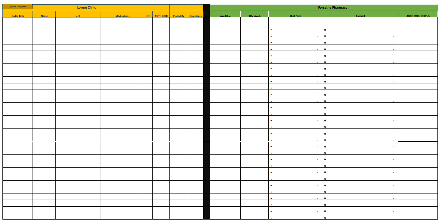
Building a Row-by-Row Order Tracker: A Spreadsheet That Behaves Like a Mini-App
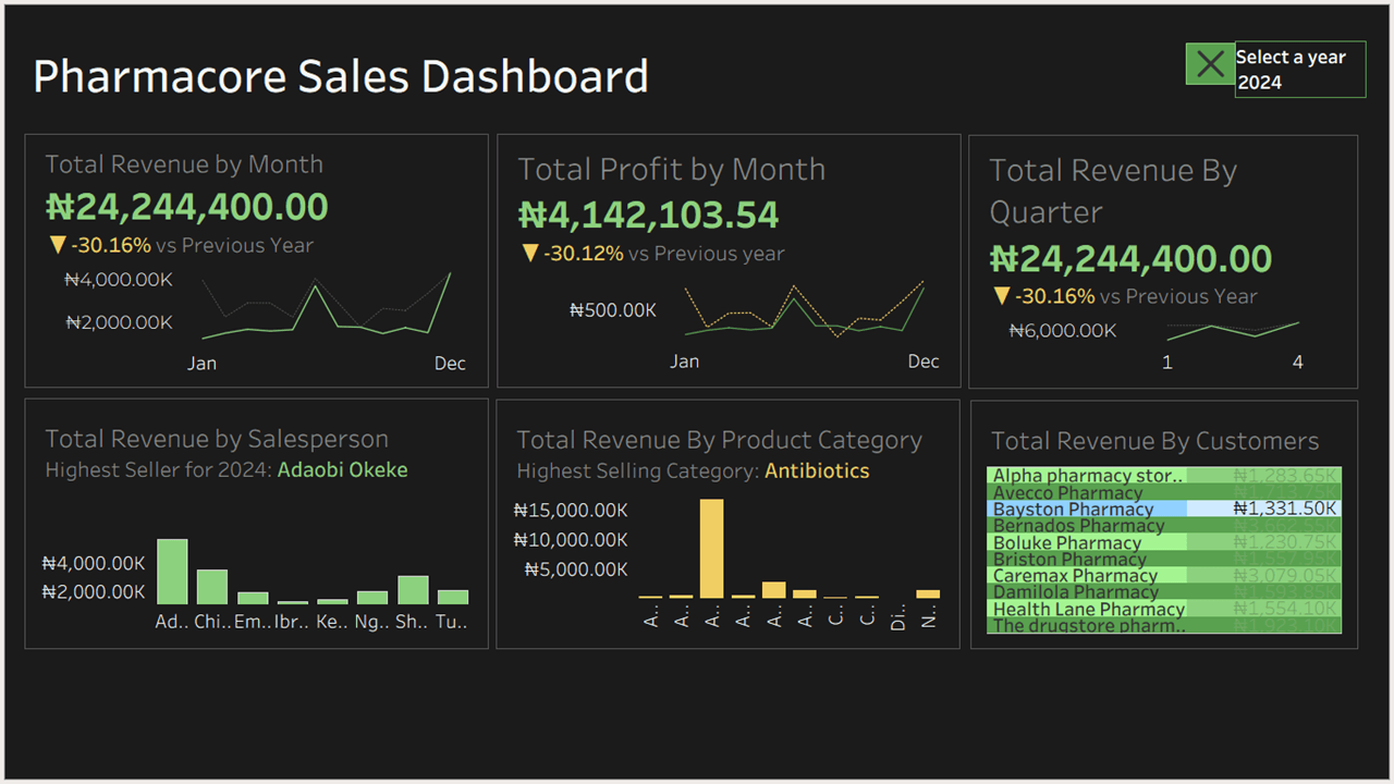
Pharmacy Distribution Visualizaton in Tableau.
Have a data story to shape?
Let's collaborate on a clear analytical product.
Get in touch